
I often get asked what method I use to calculate the frontal axis of an electrocardiogram, and I usually just say that I check if the computer’s numbers look correct and within the right quadrant.
The easiest methods of determining the frontal axis don’t necessitate the use of a scientific calculator. The quadrant method just uses the predominant polarity of leads I, II, and aVF. One can also estimate the frontal axis by using the most isoelectric limb lead and the most positive limb lead. Really, all you have to do is to find out if the patient has a normal axis, left axis deviation, right axis deviation, or extreme axis deviation. It won’t matter clinically if you’re off by a few degrees.
I started writing this post because I was reminded of an equation that was (and still is being) passed around by trainees.
I am not going to write the equation down here. I have no idea how it was derived. And I have not seen any text referencing it.
I have, however, read quite recent papers discussing the trigonometry involved.
Those of us who still remember trigonometry will attack the problem by getting the values of lead I and aVF and use these in an arctangent equation:
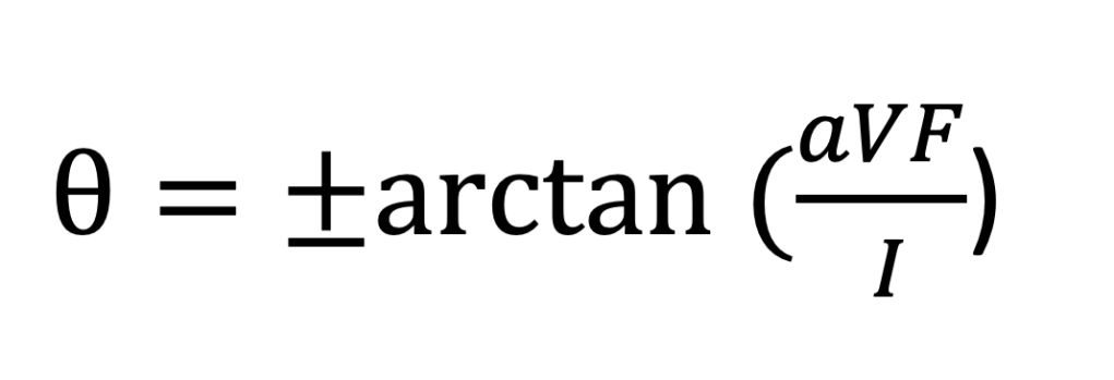
Confused? Let’s break it down.
Back to Basic Trigonometry
To illustrate, let’s review basic trigonometry and then let’s dicuss the example given to us by Novosel et al in their response to an article of Dahl and Berg.
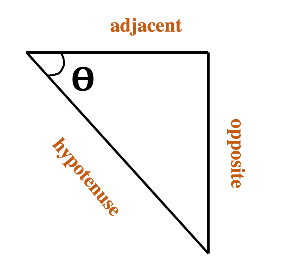
In determining the two other angles of a right triangle (remember those?), we use the ratios of the different sides. Given an angle theta θ, the ratio of the opposite side and the hypotenuse is the sine. The ratio of the adjacent side and hypotenuse is the cosine. And the ratio of the opposite side and adjacent side is the tangent. To get the angle θ from known ratios, you use the inverse functions of these — either the arc sine, arc cosine, or the arc tangent (depending on which measurements you have of course). See FIGURE 1.
We can use trigonometry by plotting out the measurements of leads I and aVF. We will be determining the angle theta θ of a right triangle formed by the frontal axis (the hypotenuse), aVF (the side opposite to theta), and lead I (the side adjacent to theta). To get the angle, we get the arctangent of aVF/lead I. See FIGURE 2.
So the equation is:

This was one of the equations used by Madanmohan et al their 1991 paper.
But there is a catch.
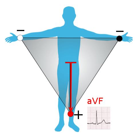
aVF is an augmented lead and is thus a unipolar lead. It is derived by making the left arm and right arm electrodes the negative pole and the foot electrode as the positive pole. Being unipolar, aVF has a different “strength” than leads I, II, and III (bipolar leads). See FIGURE 3.
Recalculating aVF
Let’s use Novosel et al’s example in their letter in Physiology News Magazine entitled “Visualizing the Novosel Formula: Comments on Dahl and Berg’s A for the mean electrical axis of the heart.”
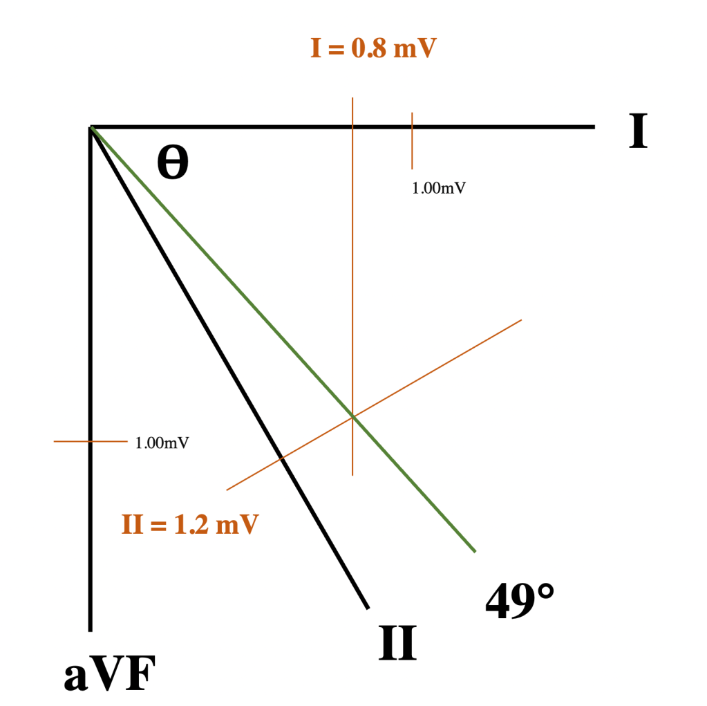
Let’s say we have an ECG with the following measurements for a particular ECG: Lead II is 1.2mV, lead I is 0.8 mV, and lead aVF is 0.8 mV.
If we are to derive the angle using leads II and I, we can use the equation first used by Madanmohan et al in their 1990 paper.
The equation they used was:
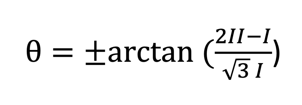
Again this was using trigonometric principles, and the answer for our particular case is 49 degrees. See Figure 4.
But remember that aVF has a different strength as leads II and I.
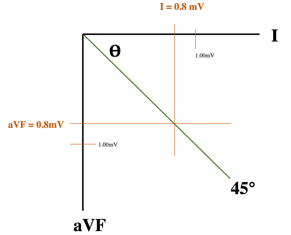
If we will use the original equation using aVF and I, we will get a different answer (i.e. 45 degrees). See FIGURE 5.
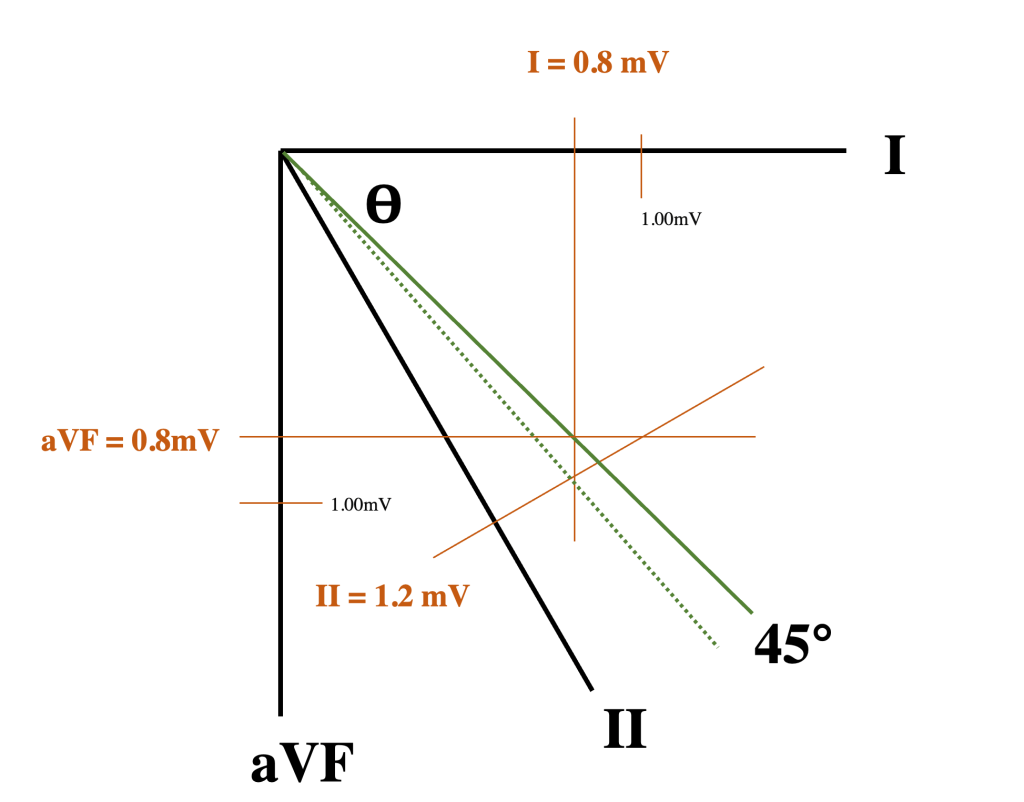
Clinically, this won’t make a difference, but if we want to be more accurate, we have to use a correction factor to take the differences between unipolar leads and bipolar leads into consideration.
The final equation with the correction factor is thus:
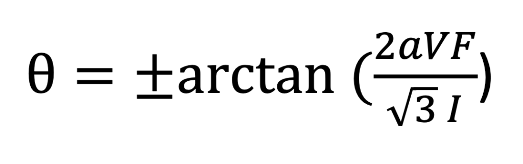
And the answer is the same now whether you use Madanmohan’s lead I and II equation or Novosel’s lead aVF and I equation (i.e. 49 degrees). See FIGURE 6.
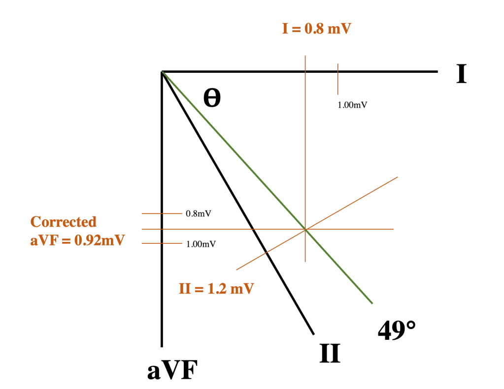
Novosel et al derived this equation by using Madanmohan’s lead II and lead I equation and Einthoven’s principles (that is, knowing that lead II can be expressed as aVF plus half of I).
If you want to see how Dahl and Berg derived it, you can download their online supplement here.
Hopefully, more work will be done on this subject so we can standardize how we measure the QRS axis and move on from the mathematics.
Sources:
1. Madanmohan BA, Saravanane C. A new method for quick and accurate calculation of the cardiac axis. Med Sci Res. 1990; 18: 933-934.
2. Madanmohan BA, Sethuraman KR, Thombre DP. A formula for quick and accurate calculation of cardiac axis from leads I and aVF. Med Sci Res. 1991; 19: 313-314.
3. Novosel et al. Corrected formula for the calculation of the electrical heart axis. Croat Med Journal. 1999 Mar;40(1):77-9. [link]
4. Dahl R and Berg R (2020). Trigonometry of the ECG. A formula for the mean electrical axis of the heart. Physiology News 120, 25-27. [link]
5. Novosel et al (2021). Visualising the Novosel Formula: Comments on Dahl and Berg’s A for the mean electrical axis of the heart. Physiology News Magazine. [link]
